Before numerical modelling was invented in the 1950s, weather forecasting was subjective and based on empirical rules. If the barometer was dropping, low pressure was on the way. Thankfully things have moved on considerably since then.
The development of numerical forecasting systems made it possible to model the movement of the atmosphere, theoretically providing a deeper understanding of what weather events were likely in the near future.
The problem is that numerical forecasts are often wrong. This is mainly because of poor understanding of the natural volatility (chaos) inherent in the atmosphere and the relatively limited number of observations used to understand the natural state of the atmosphere.
In order to create any numerical forecast, you first need to create a set of initial conditions – a three-dimensional approximation of the atmosphere “right now”. To do this, a model starts with standard weather observations, which it superimposes on to a grid.
Once the forecasting system has an initial state, it uses the equations of motion and other time-dependent equations to determine how the atmosphere will evolve over time. In other words, it creates a forecast.
This is called a deterministic forecast: a single set of inputs results in a single set of outputs.
However, this approach leaves the user exposed to volatility that it is impossible to estimate from the output of the model. All a user sees is, for example, an expected temperature of 22ºC.
This is where ensemble forecasting come in, to significantly improve the understanding of the volatility in the atmosphere. The initial conditions described above are altered slightly or “perturbed”. Then the forecast is run multiple times.
Imagine a particular observation point is capable of observing temperature to a granularity of 0.5ºC. This is good enough for most uses, but for a forecast system a difference of around 1ºC from the coolest to warmest possible temperatures is substantial.
In order to estimate within this potential difference, ensemble forecasting systems will tweak the most likely observation slightly a number of times, running the forecast model in the same way. The difference is that now, instead of the system producing a single answer, it produces a range of possibilities.
Satellite data is used to create the initial conditions for models, including cloud top temperatures and atmospheric water vapour information. Specialised satellites can also use the ripples on water surfaces to estimate wind speeds. These remotely sensed observations are secondary to “on site” observations and are used when these “normal” observations are not available.
The primary benefit of ensemble forecasting is that it provides the user with a measure of objective forecast certainty. Because the model is run multiple times, the output is a range of possibilities. This measure of certainty is particularly useful for severe weather prediction, because the costs associated with these events can be significant.
Imagine that a windfarm’s safe operating window is up to a wind speed of 40km/h.
If the forecast is for 35km/h, no alert would be triggered, but in reality there may be a 30 per cent probability of winds exceeding this safety threshold. That is, in three out of every ten similar circumstances the winds would damage the turbines. A deterministic forecast would not provide warning of this.
For windfarm operators, understanding this risk and making contingency plans can save a great deal of time and money.
Similarly, if a user is particularly concerned about the probability of heavy rain, the forecast range can be compared with this threshold to give a probability of it being exceeded. This helps the user to clearly understand what the risk is for them.
During winter when icing and snow is important, a user can use range data to provide the worst-case scenario forecast. When looking at longer range forecasts, say over five or ten days, range data also allows us to track each of the possible solutions, to see whether they agree and if or where they differ significantly.
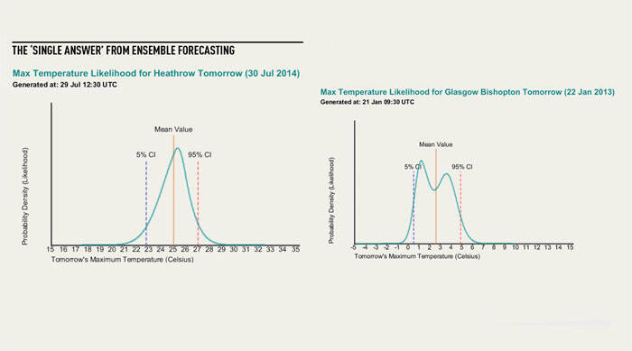
Another application of ensemble forecasting is in cases where a very accurate “single answer” is needed. Ensemble models can help users understand the probability density function, or spread of what is likely. This calculation usually results in a single most likely solution, as in the graphs, right.
Ensemble forecasting has primarily been adopted by users interested in the weather forecast more than five days ahead, mostly organisations involved in the energy industry, including generation and trading.
However, it is becoming increasingly popular with a broader range of industries from logistics planners to stock co-ordinators, to food producers and farmers, partially due to its ability to forecast the risk of exceeding a certain threshold, be it temperature, wind speed or rainfall.
Ensemble forecasting allows a user to fully understand the risks they are being exposed to, whether the risk of missing a trading opportunity or the risk of damage.
While the “most likely” forecast will always remain fundamental, understanding the range of what is likely will be increasingly applied to good planning.
Ensemble forecasts have also extended the working range of forecasts, now making it possible to make decisions based on signals in the data up to ten or even 15 days ahead of a potential event.
This horizon is constantly being pushed back, with increasingly accurate results coming from the monthly forecasts systems, allowing us to understand the outline of what the overall weather patterns will look like up to a month or more in advance, something that was previously thought impossible.
Byron Drew, Lead Forecaster EMEA, Metra Weather